How Diffusion Policy
Training Actually Works

We pick one concrete example — Episode 0, frames 4 & 5 — and trace it end-to-end through every step of the training pipeline with real numbers.

Live Data: so101_pick_place_red_cube • Episode 0 • Frames 4–5
Scroll to begin ↓
0

Your Dataset

10 teleoperation demonstrations of an SO-101 robot picking and placing a red cube

10
Episodes
9,219
Total Frames
30
FPS
6
DOF Joints
2
Cameras
640×480
Resolution
Front Camera
observation.images.front
Side Camera
observation.images.side

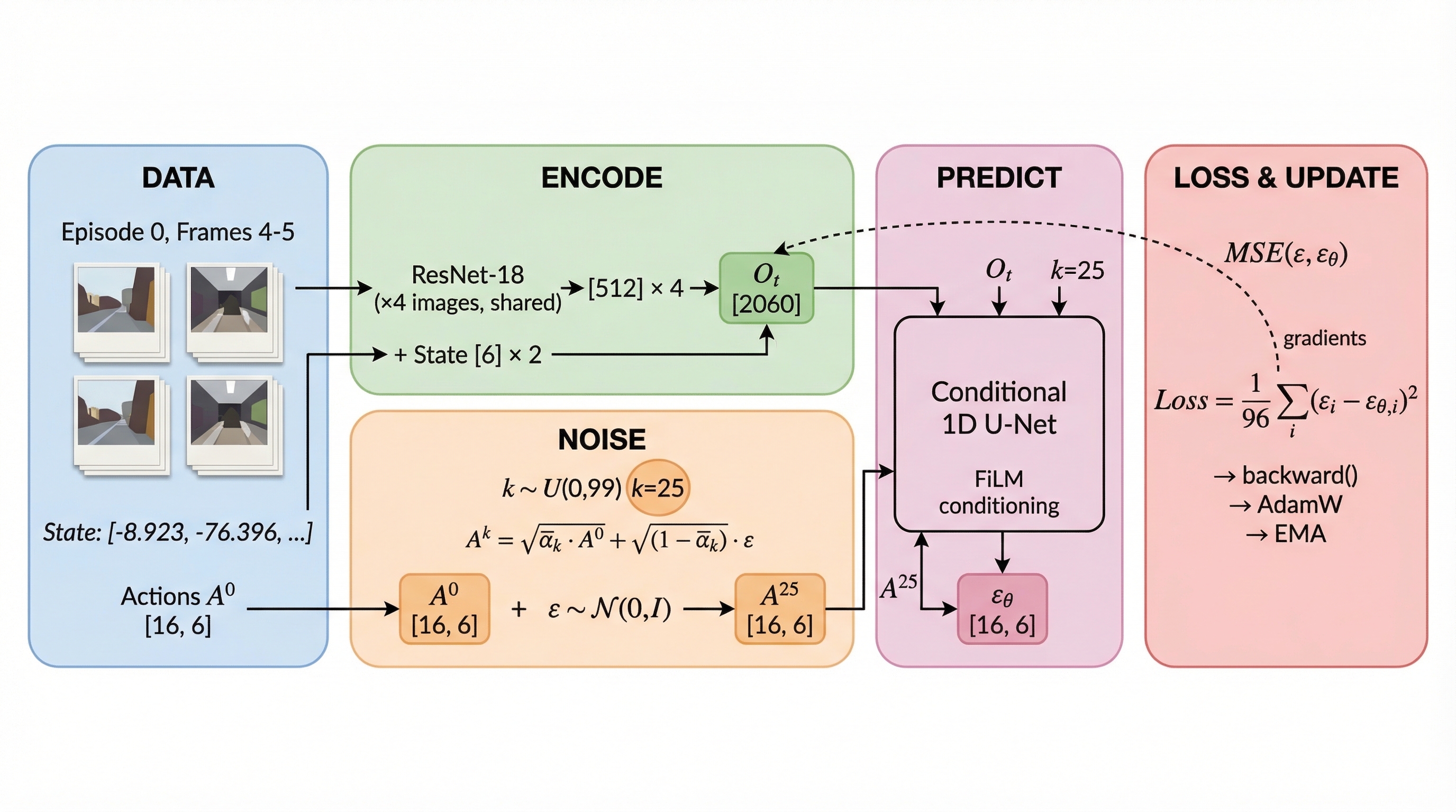
We'll trace one training example through the entire pipeline: Episode 0, frames 4 & 5 (timestamps 0.133s and 0.167s). Every number you see below comes from this exact data point.

1

Here Are Your Two Observation Frames

The policy sees exactly To = 2 frames: frame 4 (t−1) and frame 5 (t) from Episode 0

Front Camera — observation.images.front

These are the actual camera images the robot saw. Two consecutive frames give the network a sense of motion.

Frame 4 (t−1) — t = 0.133s ot-1
Frame 5 (t) — t = 0.167s ot
Side Camera — observation.images.side
Frame 4 (t−1) — t = 0.133s ot-1
Frame 5 (t) — t = 0.167s ot

Two cameras × two timesteps = 4 images total feeding into the vision encoder. Each image is [480, 640, 3] RGB.

# Extract T_o=2 consecutive frames for both cameras # Episode 0, frames 4 and 5 (timestamps 0.133s and 0.167s at 30 FPS) obs_t_minus_1 = { 'front': dataset[4]['observation.images.front'], # [480, 640, 3] 'side': dataset[4]['observation.images.side'], # [480, 640, 3] 'state': dataset[4]['observation.state'], # [6] } obs_t = { 'front': dataset[5]['observation.images.front'], # [480, 640, 3] 'side': dataset[5]['observation.images.side'], # [480, 640, 3] 'state': dataset[5]['observation.state'], # [6] }
2

Here Is the Proprioceptive State

6 joint angles read from the robot's encoders — the robot's internal sense of where it is

observation.state — Frame 4 (t−1) vs Frame 5 (t)
JointIndexFrame 4 (t−1)Frame 5 (t)Δ (Change)
Shoulder Pan0 -8.923° -9.099° -0.176°
Shoulder Lift1 -76.396° -76.396° 0.000°
Elbow Flex2 77.670° 77.758° +0.088°
Wrist Flex3 8.659° 6.549° -2.110°
Wrist Roll4 122.945° 122.945° 0.000°
Gripper5 6.560° 6.560° 0.000°
What the Policy Receives
State vector at t−1 (Frame 4):
st-1 = [-8.923, -76.396, 77.670, 8.659, 122.945, 6.560]
State vector at t (Frame 5):
st  = [-9.099, -76.396, 77.758, 6.549, 122.945, 6.560]
Concatenated state input:
[st-1, st] → 12 values total (6-dim × 2 frames)

Between frames 4→5 (33ms apart), the shoulder pan, elbow, and wrist flex are moving — the robot is adjusting its arm. The shoulder lift, wrist roll, and gripper are stationary. Two frames give the network a sense of velocity.

3

Here Are the 16 Actions to Predict

The prediction horizon Tp = 16 — starting at frame 5, these are the next 16 target joint positions

Action Chunk A&sup0; — Shape: [16, 6]

In this early phase of Episode 0, the robot is converging to its initial position. All 16 actions are identical — the teleoperator's leader arm is holding steady. This is A&sup0; — the clean action trajectory before any noise is added.

Step Shoulder Pan Shoulder Lift Elbow Flex Wrist Flex Wrist Roll Gripper
Why Are They All The Same?

At the very start of a teleoperation episode, the operator positions the leader arm and waits. The action column records the leader's (target) position at every frame. Since the leader isn't moving yet, frames 0–59 all have the same action: [-10.374, -81.670, 77.846, 2.681, 123.209, 6.495]. Later in the episode, the actions diverge as the robot begins its pick-and-place motion.

# Extract T_p=16 consecutive actions starting at frame 5 action_chunk = [] for i in range(16): idx = min(5 + i, len(episode) - 1) action_chunk.append(episode[idx]['action']) A_0 = torch.stack(action_chunk) # shape: [16, 6] # All 16 rows are [-10.374, -81.670, 77.846, 2.681, 123.209, 6.495]
4

Passing Images Through the ResNet Encoder

4 images go through a modified ResNet-18 with SpatialSoftmax → 4 × [64] feature vectors → concatenate with state

Architecture Overview
ResNet-18 Encoder Architecture — 4 images through shared-weight ResNet-18 with SpatialSoftmax to Global Conditioning Vector [268]
Tracing Real Pixel Values — Front Camera, Frame 5 (t)

Let's trace actual pixel values from the frame we extracted in Step 1. We sample the center pixel and show what happens at each processing stage.

Sampled Pixel (center of frame)
Red crosshair shows the sampled pixel location (320, 240)
RGB Values at (320, 240)
Loading pixel values from video frame...
Step-by-Step: Real Numbers Through Each Layer

Here's what happens to our front camera frame (t=0.167s) as it passes through each ResNet layer. We show the tensor shape at each stage, and for the first two stages, the actual numerical values at our sampled pixel.

Input (raw frame)
[3, 480, 640]
pixel[320,240] = [R, G, B] (loading...)
Resize + CenterCrop
[3, 76, 76]
480×640 → scale to 76×101 → center crop to 76×76.
pixel values preserved (nearest-neighbor or bilinear)
ImageNet Normalize
[3, 76, 76]
normalized = (pixel/255 - mean) / std (loading...)
conv1(3→64, 7×7, stride 2, pad 3)
[64, 38, 38]
64 learned 7×7 filters convolve over the 3-channel input. Each output is a dot product of a 7×7×3 = 147-element patch with a learned kernel.
GroupNorm(4, 64) + ReLU
[64, 38, 38]
64 channels split into 4 groups of 16. Each group normalized independently. ReLU zeros negative values.
MaxPool2d(3, stride 2, pad 1)
[64, 19, 19]
Take max in each 3×3 window, stride 2 → halve spatial dims
layer1: BasicBlock(64→64) × 2
[64, 19, 19]
Each block: conv3×3 → GN → ReLU → conv3×3 → GN + skip. 2 blocks = 8 conv layers.
layer2: BasicBlock(64→128, stride 2)
[128, 10, 10]
Downsample 2× + double channels. ~23,000 activations.
layer3: BasicBlock(128→256, stride 2)
[256, 5, 5]
Downsample again. ~6,400 activations encode mid-level features.
layer4: BasicBlock(256→512, stride 2)
[512, 3, 3]
Final conv layers. 512 × 3 × 3 = 4,608 high-level features.
Conv2d(512→32, 1×1)
[32, 3, 3]
Project 512 channels down to 32 keypoint heatmaps.
SpatialSoftmax → Expected (x, y)
[32, 2]
Softmax over each 3×3 heatmap → weighted average of (x, y) coordinates. Each keypoint becomes a 2D position.
Flatten
[64]
32 keypoints × 2 coordinates = 64-d vector summarizing the entire 480×640 image.
All 4 Images → Global Conditioning Vector Ot

The same shared-weight ResNet-18 + SpatialSoftmax processes all 4 images (2 cameras × 2 timesteps). Each produces a [64] vector (32 keypoints × 2 coords). These are concatenated with the two state vectors from Step 2.

ffront,t-1
[64]
fside,t-1
[64]
ffront,t
[64]
fside,t
[64]
st-1
[6]
st
[6]
↓ Concatenate & Flatten
Global Conditioning Vector Ot
Shape: [B, 268]
(64 × 4 images) + (6 × 2 states) = 256 + 12 = 268
Concrete values for the state portion (from Step 2):
Ot[256:262] = st-1 = [-8.923, -76.396, 77.670, 8.659, 122.945, 6.560]
Ot[262:268] = st  = [-9.099, -76.396, 77.758, 6.549, 122.945, 6.560]
Why SpatialSoftmax Instead of Global Average Pooling?

Standard ResNet-18 uses AdaptiveAvgPool which discards all spatial information. For robot manipulation, where objects are matters just as much as what they are. SpatialSoftmax learns 32 keypoints — each one a (x, y) coordinate localizing a salient feature in the image. This preserves spatial structure in a compact 64-d vector. GroupNorm replaces BatchNorm because robot learning uses small batch sizes: GroupNorm(num_features // 16, num_features).

# Modified ResNet-18: BatchNorm → GroupNorm, SpatialSoftmax pooling resnet = models.resnet18(weights='IMAGENET1K_V1') resnet.avgpool = nn.Identity() # Remove global avg pool resnet.fc = nn.Identity() # Remove classifier head def replace_bn_with_gn(module): for name, child in module.named_children(): if isinstance(child, nn.BatchNorm2d): num_ch = child.num_features setattr(module, name, nn.GroupNorm(num_ch // 16, num_ch)) else: replace_bn_with_gn(child) replace_bn_with_gn(resnet) # SpatialSoftmax: 512-ch feature maps → 32 keypoints × 2 coords spatial_softmax = SpatialSoftmax( input_shape=[512, 3, 3], num_kp=32, # 32 learned keypoint detectors ) # output: [B, 32, 2] → flatten → [B, 64] # Forward pass with our 4 images images = torch.stack([front_t1, side_t1, front_t, side_t]) # [4, 3, 76, 76] feat_maps = resnet(images) # [4, 512, 3, 3] features = spatial_softmax(feat_maps).flatten(1) # [4, 64] # Combine with proprioceptive state state_feats = torch.cat([state_t1, state_t]) # [12] O_t = torch.cat([features.flatten(), state_feats]) # [268]
5

Adding Noise to the Actions

Pick diffusion timestep k = 25 and corrupt the clean actions with Gaussian noise

The Forward Diffusion Formula
$$A^k = \sqrt{\bar{\alpha}_k} \cdot A^0 + \sqrt{1 - \bar{\alpha}_k} \cdot \epsilon, \quad \epsilon \sim \mathcal{N}(0, I)$$
Computing ā₂₅ with the Cosine Schedule
Cosine schedule formula:
$$f(t) = \cos\!\left(\frac{t/T + 0.008}{1.008} \cdot \frac{\pi}{2}\right)^{\!2}, \quad \bar{\alpha}_k = \frac{f(k)}{f(0)}$$
At k = 25 (out of 100 total steps):
Plugging In Real Numbers — Joint 0 (Shoulder Pan)
Clean action: A&sup0;[0] = -10.374
Sampled noise: ε[0] = 0.730
ā₂₅ ≈
Full 6-Joint Noise Addition at k = 25
JointA&sup0; (clean)ε (noise)√ā × A&sup0;√(1-ā) × εA²⁵ (noisy)
Interactive: Noise Level vs Diffusion Timestep

Drag the slider to see how increasing k destroys the action signal. At k=0, actions are clean. At k=99, pure noise.

Diffusion Timestep k 25
āk =
SNR =
Noise Schedule: Cosine (Squared) — 100 Steps
from diffusers import DDPMScheduler noise_scheduler = DDPMScheduler( num_train_timesteps=100, beta_schedule='squaredcos_cap_v2', prediction_type='epsilon', ) A_0 = action_chunk # [B, 16, 6] eps = torch.randn_like(A_0) # [B, 16, 6] k = torch.tensor([25]) # diffusion timestep # A_25 = sqrt(alpha_bar_25) * A_0 + sqrt(1 - alpha_bar_25) * eps A_25 = noise_scheduler.add_noise(A_0, eps, k)
6

The Diffusion Timestep Embedding

The integer k = 25 gets encoded into a rich 256-dim vector via sinusoidal frequencies, then processed by an MLP

Sinusoidal Position Encoding for k = 25
128 log-spaced frequencies:
$$\text{freq}_j = \exp\!\left(-j \cdot \frac{\ln(10000)}{127}\right), \quad j = 0, 1, \ldots, 127$$
256-dim embedding:
$$\text{emb} = [\sin(25 \cdot \text{freq}_0),\; \ldots,\; \sin(25 \cdot \text{freq}_{127}),\; \cos(25 \cdot \text{freq}_0),\; \ldots,\; \cos(25 \cdot \text{freq}_{127})]$$
The 256-Dimensional Embedding Vector for k = 25

First 128 values are sin(25 × freqj), last 128 are cos(25 × freqj). High-frequency components (left) oscillate rapidly; low-frequency components (right) change slowly.

First 5 values:
MLP Projects Embedding to Conditioning Dimension
SinusoidalPosEmb(256)
[256]
Raw sinusoidal encoding of k=25
Linear(256 → 1024)
[1024]
First projection
Mish activation
[1024]
x · tanh(softplus(x))
Linear(1024 → 256)
[256]
Timestep embedding t_emb
Full Conditioning Vector
t_emb
[256]
+
Ot
[268]
↓ Concatenate
Full Conditioning
[256 + 268] = [524]
Fed into every ResBlock via FiLM
class SinusoidalPosEmb(nn.Module): def __init__(self, dim=256): super().__init__() self.dim = dim def forward(self, x): half_dim = self.dim // 2 # 128 emb = math.log(10000) / (half_dim - 1) emb = torch.exp(torch.arange(half_dim) * -emb) emb = x[:, None] * emb[None, :] # [B, 128] emb = torch.cat([emb.sin(), emb.cos()], dim=-1) # [B, 256] return emb # MLP after sinusoidal encoding diffusion_step_encoder = nn.Sequential( SinusoidalPosEmb(256), nn.Linear(256, 1024), nn.Mish(), nn.Linear(1024, 256), ) t_emb = diffusion_step_encoder(torch.tensor([25])) # [1, 256] full_cond = torch.cat([t_emb, O_t], dim=-1) # [1, 524]
7

The U-Net Predicts Noise

A 1D temporal U-Net takes the noisy actions + conditioning and predicts the noise to remove

Architecture Overview
Conditional 1D U-Net Architecture — Encoder/Decoder with skip connections and FiLM conditioning
Inputs & Output
Noisy Actions A²⁵
[B, 16, 6] → rearrange → [B, 6, 16]
Full Cond
[B, 524]
↓ Fed into ConditionalUnet1D
Predicted Noise εθ
[B, 6, 16] → rearrange → [B, 16, 6]
Encoder (Downsampling Path)
Input
[B, 6, 16]
Noisy actions (channels-first)
Conv1d(6→256) + GroupNorm + Mish
[B, 256, 16]
ResBlock + FiLM(cond[524] → scale,bias[256])
↓ Downsample (stride 2)
Conv1d(256→512) + GroupNorm + Mish
[B, 512, 8]
ResBlock + FiLM(cond[524] → scale,bias[512])
↓ Downsample (stride 2)
Conv1d(512→1024) + GroupNorm + Mish
[B, 1024, 4]
ResBlock + FiLM(cond[524] → scale,bias[1024])
Bottleneck (Mid)
2× ResBlock(1024→1024, kernel=5)
[B, 1024, 4]
Conv1d + GroupNorm + Mish + FiLM, no spatial change
Decoder (Upsampling Path + Skip Connections)
Upsample + Cat(skip) → Conv1d(1024+1024→512)
[B, 512, 8]
Skip from encoder level 3
Upsample + Cat(skip) → Conv1d(512+512→256)
[B, 256, 16]
Skip from encoder level 2
Cat(skip) → Conv1d(256+256→256) → Conv1d(256→6)
[B, 6, 16]
Final projection to action dim
Rearrange [B, 6, 16] → [B, 16, 6]
[B, 16, 6]
Predicted noise εθ
FiLM Conditioning — How Observations Guide Denoising
At every ResBlock in the U-Net:
cond [524] → Linear → [2 × out_channels] → split into scale γ and bias β
$$\text{output} = \gamma(\text{cond}) \cdot \text{features} + \beta(\text{cond})$$
Example (first encoder block):
Linear(524 → 512) → split → γ [256] scales features, β [256] shifts features

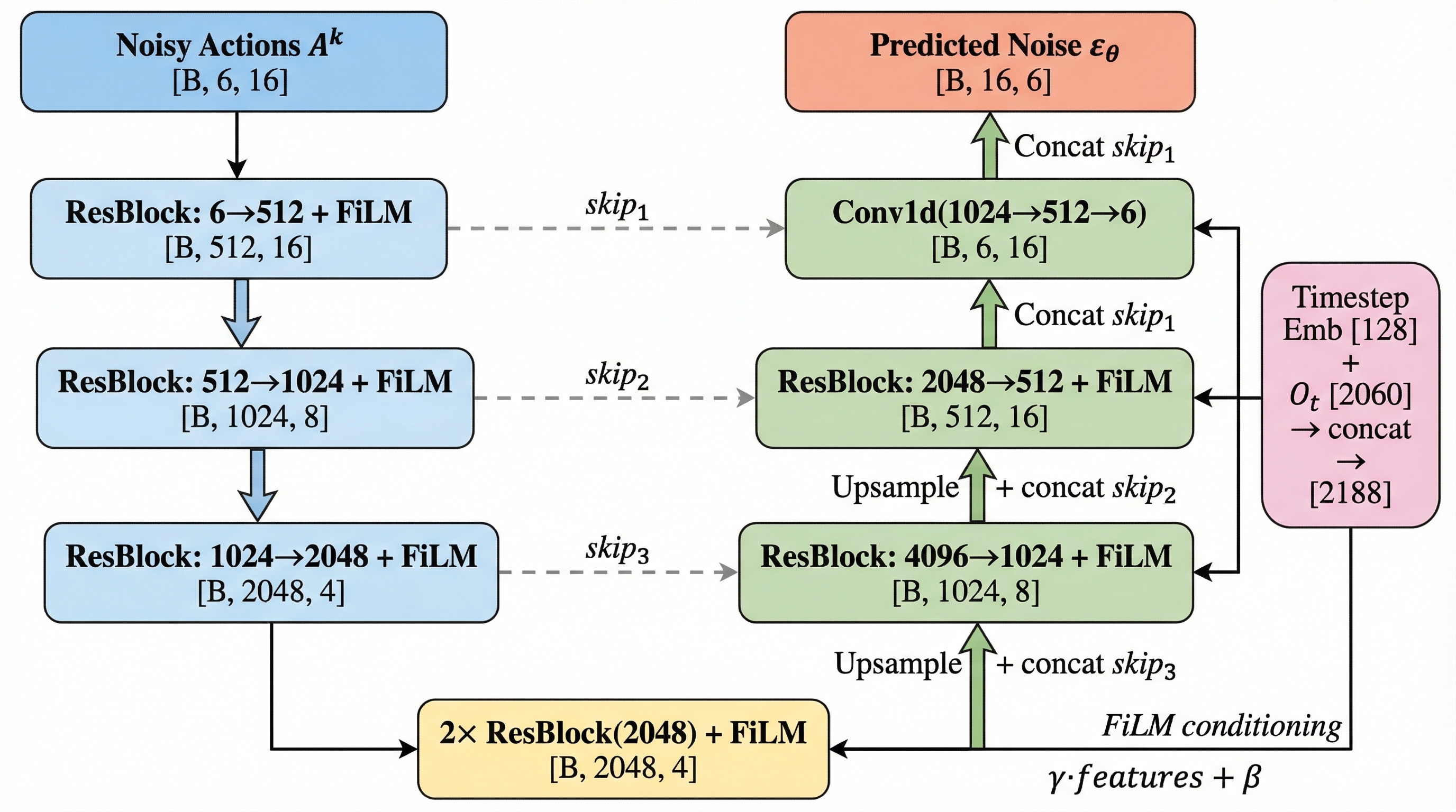
FiLM means the network doesn't just see the observation — it modulates how it processes the noisy actions at every layer. "Given what I see and which noise level we're at, here's how to denoise."

class ConditionalUnet1D(nn.Module): def __init__(self, input_dim=6, global_cond_dim=268, down_dims=[256, 512, 1024], diffusion_step_embed_dim=256): # Total cond dim = 256 + 268 = 524 # Encoder: 6→256→512→1024 # Decoder: 1024→512→256→6 ... def forward(self, sample, timestep, global_cond): # sample: [B, 16, 6] → [B, 6, 16] x = sample.permute(0, 2, 1) # Timestep embedding t_emb = self.diffusion_step_encoder(timestep) # [B, 256] cond = torch.cat([t_emb, global_cond], dim=-1) # [B, 524] # Encoder with FiLM skips = [] for resblock, downsample in self.down_modules: x = resblock(x, cond) # FiLM: Linear(524→2*ch) skips.append(x) x = downsample(x) # Bottleneck x = self.mid_modules(x, cond) # Decoder with skip connections for resblock, upsample in self.up_modules: x = upsample(x) x = torch.cat([x, skips.pop()], dim=1) x = resblock(x, cond) x = self.final_conv(x) # [B, 6, 16] return x.permute(0, 2, 1) # [B, 16, 6]
8

Computing the Loss & Gradient Update

Compare predicted noise to actual noise, compute MSE, and update all weights

Actual Noise ε vs Predicted Noise εθ (Joint 0 across 16 timesteps)

Blue = the actual Gaussian noise ε we sampled in Step 5. Coral = what the U-Net predicted. Early in training, these are very different.

MSE Loss Computation
$$\mathcal{L} = \frac{1}{96} \sum_{i=1}^{96} (\epsilon_i - \epsilon_{\theta,i})^2 \quad \text{(96 = 16 timesteps} \times \text{6 joints)}$$
Per-element squared errors (first 6 of 96):
Total MSE Loss =
Gradient Flows Back Through Everything
Loss = MSE(ε, εθ)
↑ gradients flow back
U-Net weights
All Conv1d, GroupNorm, FiLM layers
ResNet-18 weights
All conv layers, GroupNorm layers
Weight Update
AdamW step: θnew = θold − lr × m̂/(√v̂ + ε) − lr × λ × θold
Learning rate: 1e-4
EMA update: θema = 0.9999 × θema + 0.0001 × θnew

The EMA (Exponential Moving Average) model is a smoothed copy of the weights used at inference time. It prevents the deployed policy from being affected by noisy gradient updates.

Training Hyperparameters
ParameterValue
OptimizerAdamW (betas = 0.95, 0.999, weight_decay = 1e-6)
Learning Rate1e-4 with cosine annealing + 500-step warmup
Batch Size64
Epochs3000
Diffusion Steps100 (train) / 10 (DDIM inference)
EMA Decaypower=0.75, max=0.9999
Prediction Horizon Tp16
Observation Horizon To2
Action Execution Ta8 (receding horizon at inference)
# One training iteration — the complete pipeline from this walkthrough for batch in dataloader: # Steps 1-2: Extract observations (4 images + 2 state vectors) obs = batch['obs'] A_0 = batch['action'] # [B, 16, 6] — Step 3 # Step 4: Encode observations → global conditioning O_t = obs_encoder(obs) # [B, 268] # Step 5: Sample noise and random timestep eps = torch.randn_like(A_0) k = torch.randint(0, 100, (B,)) A_k = scheduler.add_noise(A_0, eps, k) # Steps 6-7: U-Net predicts noise eps_theta = unet(A_k, k, global_cond=O_t) # [B, 16, 6] # Step 8: MSE loss + backprop + update loss = F.mse_loss(eps_theta, eps) optimizer.zero_grad() loss.backward() optimizer.step() lr_scheduler.step() ema_model.step(model.parameters())

That's One Training Iteration

Everything you just saw — from raw camera frames to gradient update — happens once per batch element, thousands of times

Complete Pipeline — One Training Iteration
Complete Diffusion Policy training pipeline — from data sampling through encoding, noise addition, U-Net prediction, to loss and gradient update
At Inference Time (After Training)

The process runs in reverse: start with pure Gaussian noise AK ~ N(0, I), then iteratively denoise for K steps (or 10 DDIM steps for 10x speedup). At each step, the trained U-Net predicts the noise to subtract, conditioned on the current observation Ot. The result is a clean 16-step action trajectory. Only the first Ta = 8 actions are executed before replanning — this receding horizon approach balances temporal consistency with responsiveness.